Today we are going to talk about multigraphs and apply them to chemistry. A multigraph is just a graph in which multiple edges and loops are allowed. Multiple edges are the name for having more than one edge between two vertices, and loops are edges both of whose ends are at the same vertex. It turns out we can once again represent Lewis structures like this. A lone pair is a loop, a double bond is two edges, and a triple bond is three edges.
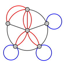
Above is a multigraph, courtesy of the great Wikipedia: http://upload.wikimedia.org/wikipedia/commons/thumb/c/c9/Multi-pseudograph.svg/220px-Multi-pseudograph.svg.png.
Note that you have the red multiple edges and the blue loops.
So what are the properties of a mutigraph we are concerned with? Once again we have vertices, edges, and degree. The vertices are the gray dots in the above diagram, and the edges are the black, red, and blue in the diagram. Degree is defined to be the number of edges adjacent to a vertex, where loops are counted twice, one for each end. In this way the sum of all degrees is still twice the number of vertices.
This is nice. For starters we can represent any Lewis structure much more completely with this convention. Graph theoretic properties once again have interesting meanings. Every edge still represents an electron pair. The degree of a vertex still represents the number of electrons in its valence shell after bonding, where loops are counted twice for a vertex. Formal charge has an interesting representation now. It is the difference between the number of electrons present on the individual atom and the degree in the accompanying graph.
Pictures might be an excellent aid, but it’s better to construct lewis structures yourself! Draw the Lewis dot structure of your favorite compound, say glucose. Go on now. Do it on paper. Start by making a graph with the atoms as vertices. Now, turn the lone pairs into loops, so for every lone pair, drawn an edge from that lone pair’s atom to itself. Finally, draw an edge between two atoms with a single bond, draw two between two with a double bond, and draw three between two with a triple bond. There you go.
Now, once again these multigraphs can be applied to calculate the formula of certain compounds! Let’s start with hydrocarbons because they are simple. Say we have an acyclic hydrocarbon with 5 carbons and 8 hydrogens. What bonds can it have?
Note that this is an alkane so there are no cycles. There are also no lone pairs because carbon is not very electronegative and instead makes 4 bonds. The carbons in total have degree 20 because they need to be adjacent to 4 edges (electron pairs). Since 8 of these are taken up by carbon-carbon sigma bonds (there are 4, because of our tree with 4 edges, but each is counted twice for each of the carbons), and 8 by C-H bonds, C-C pi bonds are counted a total of 4 times, which means that there are 2 of them. So either there is a triple bond or two double bounds.
Let’s do another example. What does carbon monoxide look like? First, we can draw the simple graph for it, which is a carbon connected to an oxygen. The edges in the simple graph represent the sigma bonds that do not hold lone pairs, and onto them we will draw the extra multiple edges which represent pi bonds. Clearly 5 edges need to be drawn in some capacity, since we need 10 total valence electrons. 4 are for the carbon, and 6 for the oxygen. The only way to do this is to make two extra pi bonds between C and O and then give each of C,O a lone pair. So we have a graph on two vertices connected by a triple edge, each of which has a loop attached to it.
So we have seen that the idea of interpreting Lewis structures as simple graphs can be extended to interpreting them as multiple graphs. Once again, this allows us to mathematically capture the structure of many compounds and rationalize their structures to some extent using degree arguments. Once again, there is still nothing about the actual shape of the molecules involved here, but that is covered very nicely in our previous posts on Group Theory. Stay tuned for next time!
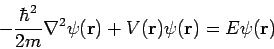

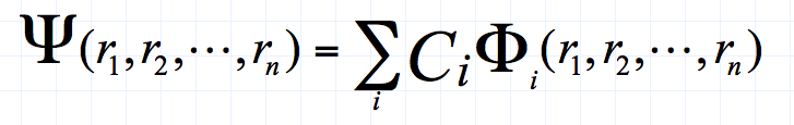
 is essentially the solution to to the electronic Schrodinger equation, producing the particular wave function that’s dependent on electrons only. The reason why this particular wave function is so useful is because by taking its partial derivatives, one can gain information about Dipole moments, polarizability, molecular structures, and even spectra: electronic, photoelectron, vibrational, rotaional, NMR, etc. If you forget, the wave equation is essentially the superposition of a bunch of states, and can be represented as:
 , specify the different quantum “alternatives” available – a particular quantum state. The partial derivatives are taken with respect to each ket, so the partial derivatives of a wave function are simply,
 , and X1, X2, …, XN, are simply the kets

 is the Hartree-Fock wave function, and
  refers to the molecular orbital i.
